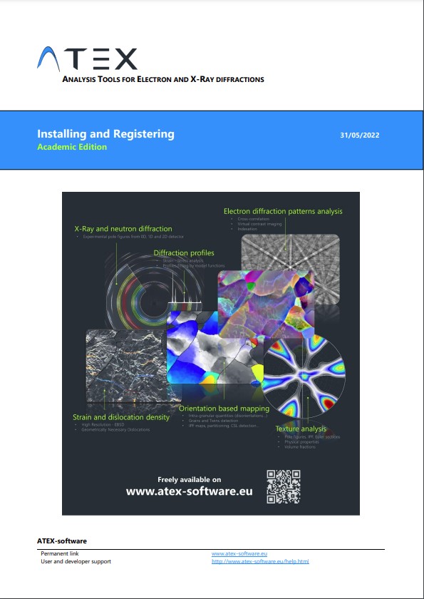
Tutorials

INSTALLATION ORIENTATIONS LIST CRYSTAL PLASTICITY
ORIENTATION RELATIONSHIP

General Help

Installing

1 - Download and install the demonstration version

- Install it on the computer you plane to use to analyze your data.
- The computer need an internet connection.
- You will also probably have to authorize your antivirus to install the program.
- Prefer an install on a computer equipped with a large screen.
- Avoid c:/program files if you are not administrator of your computer.
- If you installed ATEX on a laptop, don't forget to put your icon size to 100% and probably reboot (if you want to see correctly all the buttons).


2 - Register

- Simply fill the form correclty


3 - Updates

Click on the update button (red button), ATEX will close, and update module will open.


- Update (48Mo to download).
- When it is done, click on "open ATEX" button (the red button is not visible anymore).


For LAPTOP

If windows rescale the buttons, disable the option "Let Windows try to fix apps so they're not blurry" in Advanced scaling settings.


For Apple virtual Windows


Different types of files

A specific name of extension is associated to each kind of data, note that data can be experimental as well as simulated

Data Types File Extensions     State
Electron Backscatter Diffraction .EBSD.atex ready
Electron Backscatter Diffraction + kikuchi patterns .KIKU.atex ready
Electron Backscatter Diffraction 3D .EB3D.atex in progress
Orientations List .ORLI.atex ready
X-Ray Incomplete Pole Figures .XIPF.atex ready
X-Ray Diffraction Profiles .PROF.atex ready
X-Ray 2D Detector .X_2D.atex ready
X-Ray 2D Detector + Spatial Information .X2DX.atex in progress
Orientation Density Function (ODF) .CODF.atex ready
Raman Microscopy .RAMA.atex ready


EBSD maps

The reference system of an EBSD map is centered on the left top corner, axis 1 is directed toward the right, axis 2 toward the bottom and axis 3 toward inside the screen.

Crystal Systems
Cubic                      Hexagonal                      Tetragonal                     
Orthorhombic                      Monoclinic                      Triclinic                     

Note that if your crystal is not defined as above, it will not be recognized by ATEX, example for the tetragonal symmetry it is "c" which must be different from "a" and "b".
Ref: wikipedia, Bravais lattice

Write orientation list file in FORTRAN (*.orli.atex)

Code: (copy and past it in your code)

EBSD

Supported data files:

    *.ctf (Channel Text File) from Oxford or Bruker
    *.ang (hexagonal or square grids) from EDAX
    *.txt (custom files)


Noise reduction

The strategy to assign an orientation to non-indexed pixels is: First the non-indexed pixels surrounded by 8 indexed pixels displaying a misorientation less than 3° are indexed by the mean orientation of these 8 neighbouring pixels. Several loops are performed, until all non-indexed pixels are corrected. Then, the procedure is repeated with 7 neighbours, 6… down to 1 neighbour pixel. The procedure is stopped when all the non-indexed pixels have been corrected. Example with 6 neighbour pixels:


Spike correction

The strategy to assign a new orientation to a spike is as follows: The spikes displaying at least seven indexed neighbour pixels misoriented by less than 3° are re-oriented by the mean orientation of those 7 or 8 neighbour pixels. One or two loops can be set by the user. The procedure is limited to two loops to avoid important changes of the original map. See the figure bellow.

Example

Example

References

L. S. Tóth, P. Gilormini, J. J. Jonas, Acta Metallurgica 1988, 36, pp.3077-3091
J. Baczynski, J. J. Jonas, Acta Materialia 1996, 44, pp.4273-4288
B. Beausir, L. S. Tóth, K. W. Neale, Acta Materialia 2007, 55, pp.2695-2705
Y. Zhou, K. W. Neale, L. S. Tóth, Acta Metallurgica 1991, 11, pp.2921-2930
M. Hölscher, D. Raabe, K. Lücke, Steel Research 1991, 62, pp.567-575
B. Beausir, S. Biswas, D. I. Kim, L. S. Tóth, S. Suwas, Acta Materialia 2009, 57, pp.5061-5077

Example

Grains and Neighbours Detection

Grain Tolerance Angle and grain detection The procedure to define the grains is the following; The misorientation of each pixel with his four (north, south, east and west) neighbours is examined. When the misorientation exceeds the “grain tolerance angle”, a boundary is defined. Once all the pixels boundaries are defined, a flood-fill procedure is applied to search for sub-surfaces delimitated by a close boundary. The latter are defined as grains.

The file ATEX_OUT_InfosGrains.OUT give information about the detected grains.


First neighbours detection

If a grain displays a boundary with another grain, these two grains are called “first neighbours”. They represent a “pair” of grains, or a pair of neighbours. The four neighbouring pixels are considered (North, East, West and South). The list of the first neighbours of each grain can be found in the NEIGHBORS.OUT file; by row: ID; number of neighbours (NbNbors); ID of the neighbours (ID_Neighbors).

The file ATEX_OUT_Neighbors.OUT give information about the detected grains.


Grain sizes and grain shapes

Average grain size (for all the map) can be found in "Statistics" tab.

- "av. grain size (EqCA)" : The surface of each induvidual grain is calculated by the grain detection, then the diameter of the equivalent circle area is calculated from the formula bellow and the average of those diameters give the average grain size.

- "av. grain size (Surf)" : The surface of the map is divided by the total number of grains in the map which give the average surface of a grain, then the diameter of the equivalent circle area is calculated from the formula bellow giving the average grain size.

The grain size d is defined as follow: d = 2 * sqrt ( S / pi ). Where S is the surface of the grains.


Grain shapes: Ellipse fitting

Once the grains are detected and their gravity centres known, the grains are fitted by ellipses. From the fit the big axis a and the small axis b as well as the angle of the big axis with the direction 1 of the sample are obtained. Thus the ellipticity of each grains is calculated as follow: E = 1 - b / a
For a circle the ellipticity is zero and when a >> b the ellipticity tends to 1. Note that the grains on the map borders are not considered.

Example grains detection

Example twins detection

Intragranular disorientations

- Disorientation from gravity center orientation
    "DISOR_GRAV" map is the disorientation between the orientations of the gravity center and each pixel in the grain.
    "W1_GRAV" map is the disorientation between the orientations of the gravity center and each pixel in the grain w/r to the X-axis of the sample.
    "W2_GRAV" map is the disorientation between the orientations of the gravity center and each pixel in the grain w/r to the Y-axis of the sample.
    "W3_GRAV" map is the disorientation between the orientations of the gravity center and each pixel in the grain w/r to the Z-axis of the sample.
    "AV_GrO" map is the average per grain of the disorientation between the orientations of the gravity center orientation and each pixel in the grain.

- Disorientation from average grain orientation
    "DIS_AV" map is the disorientation between the average orientation and each pixel of the grain.
    "AV_AvO" map is the average per grain of the disorientation between the average orientation and each pixel of the grain.

Geometrically Necessary Dislocation Density
References

W. Pantleon, Resolving the geometrically necessary dislocation content by conventional electron backscattering diffraction, Scripta Materialia 2008, 58, 994-997.

Output Maps

- "GNDij", ij-components of the Nye Tensor, unit is L-1, [L] being the space units of your data file probably µm)
- "GNDnorm", entrywise norm of the Nye Tensor, unit is L-1.


Note if you want m-2 you can divide it by the lentgh of the Burgers vector 1/b*||a||

Disclination density tensor

"DCLij", ij-component of the disclination density tensor components, units is L-2
see: B. Beausir, C. Fressengeas, Disclination densities from EBSD orientation mapping
International Journal of Solids and Structures 2013, 50, pp.137-146.

Example


Theory

Single crystal rank 2 tensor:  

Single crystal rank 4 tensor:  

Polycrystal rank 2 tensor:  

Average elastic properties:  

- In KA:  

- For the polycrystal:  

Assumptions:

- Reuss (Lower Bound):  

- Voigt (Upper Bound):  

- Hill:  


Example

Example

Example

The calculation is too long to be in the movie, the maps corresponding to the different areas are automatically created at the end of the calculation.

To use the map calculator, if your computer is 64bits, you need to install the "tsc64.dll" on your computer, follow the next two steps.
for more information about this dll, follow this link https://helloacm.com/quick-tutorial-to-64-bit-tablacus-scripting-control/

1 - Download the "tsc64.dll" here: and place it where the "regsvr32.exe" is located, probably c:\windows\system32

2 - Download the install_tsc64dll.bat file here: ,right click on install_tsc64dll.bat file and execute it "as administrator"

If you want to uninstall it, download the uninstall_tsc64dll.bat file here: and execute it "as administrator"

X-Ray Measurements

Example

Corrections X-ray measurements

R. Guillen, C. Cossu, T. Jacquot, M. Francois, B. Bourniquel, J. Appl. Cryst. 1999, 32,pp.387-392
J.J. Heizmann, A. Vadon, D. Schlatter, J. Bessieres, Advances in X-ray Analysis. 1989, 32,pp.285-292

Textures Analysis

Imput data

You can plot textures from data coming from EBSD, 3D EBSD, ODF or an orientation list, the following video is the same for all these kinds of data

References

H.J. Bunge HJ, Z. Metallkde 1965, 56, pp.872-874
H.J. Bunge, 1987. Theoretical Methods of Texture Analysis. DGM Informationsgesellschaft, Frankfurt, Germany

Example

References Ideal Orientations

L. S. Tóth, P. Gilormini, J. J. Jonas, Acta Metallurgica 1988, 36, pp.3077-3091
J. Baczynski, J. J. Jonas, Acta Materialia 1996, 44, pp.4273-4288
B. Beausir, L. S. Tóth, K. W. Neale, Acta Materialia 2007, 55, pp.2695-2705
Y. Zhou, K. W. Neale, L. S. Tóth, Acta Metallurgica 1991, 11, pp.2921-2930
M. Hölscher, D. Raabe, K. Lücke, Steel Research 1991, 62, pp.567-575
B. Beausir, S. Biswas, D. I. Kim, L. S. Tóth, S. Suwas, Acta Materialia 2009, 57, pp.5061-5077

References Volume Fraction Calculation

L. Zuo, J. Muller, C. Esling, J. Appl. Cryst 1993, 26, pp.422-425
L. Zuo, J. Muller, C. Esling, J. Appl. Cryst 1994, 27, pp.358-361
L. Zuo, M. Humbert, C. Esling, J. Appl. Cryst 1993, 26, pp.302-304

Simulations

Microstructures

Textures

Generate velocity gradient for textures simulation

Properties from textures (ODF)

Theory

Single crystal rank 2 tensor:  

Single crystal rank 4 tensor:  

Polycrystal rank 2 tensor:  

Average elastic properties:  

- In KA:  

- For the polycrystal:  

Assumptions:

- Reuss (Lower Bound):  

- Voigt (Upper Bound):  

- Hill:  


Deformation texture simulations

References

A. Molinari, G. R. Canova, S. Ahzi, Acta Metall 1987, pp.2983-2994
A. Molinari, L. S. Toth, Acta Metall Mater 1994, pp.2453-2458

Tools


Theory

Let A and B two textures expressed on the basis of spherical harmonics, and the corresponding series of complex numbers.
The correlation coefficient between the two textures is then given by:


If C(l)=1 then A and B are proportional at rank l

A and B will be identical if both all C(l)=1 and all P(l)=1


In n-degrees of freedom problem, the probability that the variable be less than a certain value t0 is the student's t-distribution Q(t,n). Thus the value 1-Q(t,n) is the confidence level at which the hypothesis of a correlation due to chance is invalidated.


Correlation indicators

Texture Index:
Texture Difference Index:
V-delta Parameter:
Direct Correlation:
High Ranks:
Low Ranks:

Example: correlation between textures of an EBSD map and its subset.

Methods of discretization

- Random distribution - Number of orientations
The Euler space is randomly discretized at the chosen number of points. The volume fraction of each orientation is calculated from the ODF in a subspace having a radius depending on the maximum disorientation angle of the crystal structure and the chosen number of points.

- Fixed number of orientations
The Euler space is discretized randomly and homogeneously. Depending on the chosen number of points, a minimal disorientation between the orientations is deduced. The volume fraction of each orientation is calculated from the ODF in a subspace having as radius this disorientation.

- Regular Grid
The Euler space is discretized on a regular grid defined by the chosen angular resolution. The volume fraction of each orientation is calculated from the ODF in a subspace having as radius the chosen angular resolution.

- Random distribution - Disorientation
The Euler space is discretized randomly and homogeneously. Depending on the chosen minimal disorientation between the orientations, the number of points is deduced. The volume fraction of each orientation is calculated from the ODF in a subspace having as radius this disorientation.

- Constant weight
The Euler space is discretized on a regular grid defined by the chosen angular resolution. At each node of the grid the volume fraction of the ODF is evaluated. To represent this volume fraction, a number of orientations of constant weight are randomly generated around the node. Note that the final orientations did not lie on a regular grid.

Example

References

B. Beausir, J.-J. Fundenberger, Analysis Tools for Electron and X-ray diffraction, ATEX - software, www.atex-software.eu, Université de Lorraine - Metz, 2017
H.J. Bunge HJ, Z. Metallkde 1965, 56, pp.872-874
H.J. Bunge, 1987. Theoretical Methods of Texture Analysis. DGM Informationsgesellschaft, Frankfurt, Germany
A. Molinari, G. R. Canova, S. Ahzi, Acta Metall 1987, pp.2983-2994
A. Molinari, L. S. Toth, Acta Metall Mater 1994, pp.2453-2458
L. S. Tóth, P. Gilormini, J. J. Jonas, Acta Metallurgica 1988, 36, pp.3077-3091
J. Baczynski, J. J. Jonas, Acta Materialia 1996, 44, pp.4273-4288
B. Beausir, L. S. Tóth, K. W. Neale, Acta Materialia 2007, 55, pp.2695-2705
Y. Zhou, K. W. Neale, L. S. Tóth, Acta Metallurgica 1991, 11, pp.2921-2930
M. Hölscher, D. Raabe, K. Lücke, Steel Research 1991, 62, pp.567-575
B. Beausir, S. Biswas, D. I. Kim, L. S. Tóth, S. Suwas, Acta Materialia 2009, 57, pp.5061-5077
L. Zuo, J. Muller, C. Esling, J. Appl. Cryst 1993, 26, pp.422-425
L. Zuo, J. Muller, C. Esling, J. Appl. Cryst 1994, 27, pp.358-361
L. Zuo, M. Humbert, C. Esling, J. Appl. Cryst 1993, 26, pp.302-304
R. Guillen, C. Cossu, T. Jacquot, M. Francois, B. Bourniquel, J. Appl. Cryst. 1999, 32,pp.387-392
J.J. Heizmann, A. Vadon, D. Schlatter, J. Bessieres, Advances in X-ray Analysis. 1989, 32,pp.285-292
M. Dahms and H. J. Bunge, J. Appl. Cryst. 1989 22, pp.439-447
Z. Liang, J. XU, F. Wang, Mat. Sc. Eng. 1983, 60, pp.59-63
M. Humbert, F. Wagner, R. Baro, Texture of Crystalline Solids 1978, 3, pp.27-36
M. Humbert, F. Wagner, Textures and Microstructures 1987, 7, pp.115-129
P.I. Welch, Textures and Microstructures 1980, 4, pp.99-110
L.S. Toth and P. Van Houtte, Textures and Microstructures 1992, 19, pp.229-244
H.J. Bunge, Texture of Crystalline Solids 1977, 2, pp.169-174
F. Wagner,M. Humbert, J. Muller, C. Esling, Europhys. Lett. 1990, 11 (5), pp.479-483
F. Langouche, E. Aernoudt, P. Van Houtte, J. Appl. Cryst. 1989, 22, pp.533-538
A. Kudlicki, M Rowicka, M Gilski, Z. Otwinowski, J. of Applied Cryst. 2005, 38, pp 501-504

Contact

This software is developped by

Jean-Jacques Fundenberger and Benoit Beausir


contact@atex-software.eu

Location